Introduction of Clustering

Clustering is a process of grouping similar objects together. It belongs to unsupervised learning, as it’s unlabeled. There is a set of different clustering method, including partitioning method (flat clustering), hierarchical clustering and density-based method.

To measure the similarity between two objects, we can use different criteria corresponding to each specific problem.

If the object is represented as a vector: measure similarity by cosine similarity, ranging from -1 to 1.

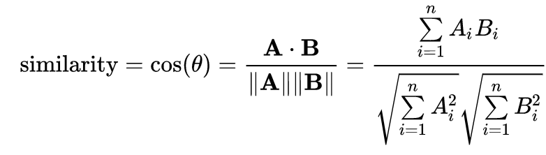
To keep a positive distance, we can use cosine distance: Dist(A,B) = 1- sim(A,B), so the range will be [0, 2]. So if two objects are getting close, its cosine distance will be close to 0. Otherwise, it will gradually increase to 2.

If the objects are sets: measure similarity by Jaccard Distance.

If the objects are points: measure similarity by Euclidean Distance. dist(x,y)² =∑_j=1ⁿ(x_j −y_j)

K-means

In this post, we mainly talk about k-means clustering, which is about iteratively assigning and recalculating the closest points to corresponding centroid until there is no difference between two iterations. It mainly contains 4 steps:

1. randomly pick K points from your sample data as initial centroids (μ_k)
2. assign each sample point to the nearest centroid
3. recalculate the centroid in each new cluster
4. repeat step 2 and 3 until cluster assignment do not change or a certain user-defined requirements have been reached. Thus, we can define the object function as: J = ∑_i=1^N∑_k=1^Kr_ik||x_i −μ_k||², r_ik means if x_i has been assigned to cluster k, then it equals 1; otherwise, it equals 0. It’s very straight forward. In each cluster, we want to minimize the sum of the squared distance of each data to the centroid. In order to obtain the smallest J, in each iteration, we will have 2 steps. One is keeping μ_k fixed, to minimize J with respect to r_ik; the other is making r_ik fixed, and minimize J with respect to μ_k. This two-step of updating μ_k and r_ik correspond to the expectation and maximization process of EM algorithm, which we will talk in later posts.

Key Problems

There are three key points of this algorithm:

• how to decide the size of K
• which K points should be chosen initially?
• when to stop the iterations

Size of K

One way to find the optimal K is to use elbow method, by increaseing the size of k gradually to find out at which point the calculated SSE will increase most rapidly.

For example, we have a dataset shown in Fig. 1. Intuitively, we can tell there are 3 clusters. We can also get the number 3 by conducting the elbow method (shown in Fig.2).

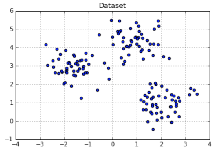
Figure 1. Dataset Example

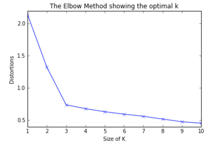
Figure 2. Elbow Result1

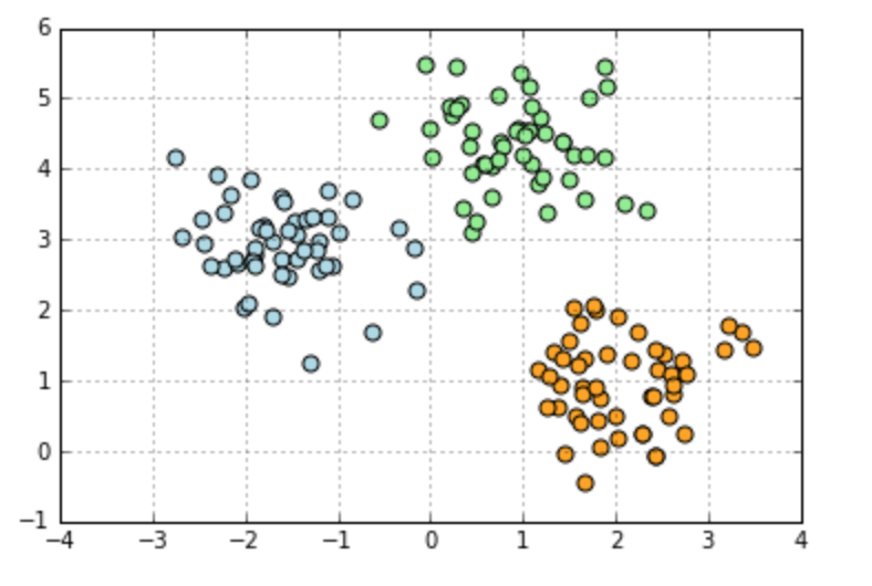
Figure 3. Clustering Result

The other way to find K is calculating silhouette coefficient. It measures how tightly within each clusters are and how seperately among different clusters. sⁱ = (bⁱ - aⁱ)/ max{bⁱ, aⁱ}

The mean intra-cluster distance (aⁱ) is the average distance between a point xⁱ and all other points in the same clusters (measures cohesion). The mean nearest-cluster distance (bⁱ) is the avg distance between xⁱ and all samples in the nearest cluster (measures seperation). It ranges from -1 to 1. The larger silhouette coefficient is, the better samples have been clustered.

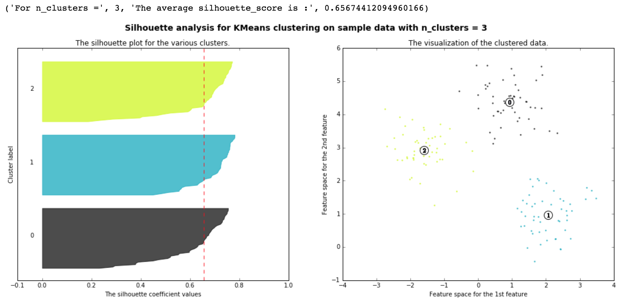
Figure 4. silhouette coefficient

Which K points to choose

One way is to randomly choose k points from your sample. However, it may lead to slow convergence. Also, the final output will be different, if you select different k points. So this algorithm lacks consistency. To solve this, an updated version of kmeans is introduced, which is kmeans++.

Kmeans++ algorithm:

1. Initialize an empty set M to store the k centroids being selected.
2. Randomly choose the 1st centroid μ_j from the input samples and assign it to M .
3. For each sample x_i that is not in M, find the minimum squared distance dist(x_i,M)² to any of the centroids in M .
4. To randomly select the next centroid μ_j , use a weighted probability distribution equal to d(μ_j,M)² /∑d(x_i ,M)²
5. Repeat steps 2 and 3 until k centroids are chosen.
6. Proceed with the classic k-means algorithm. Kmeans++ also outperforms kmeans in other aspect. Some may suggest to choose k far away points as initial points. However, this may not be a good solution when you have outliers in your dataset. In kmeans++, you can notice that it tries to choose next centroids from far-away clusters, not choose the farest point.

Common Stopping Point

1. no further changes between two iterations
2. limitation of number of iteration

Reference

[1]. https://en.wikipedia.org/wiki/Cosine_similarity

[2]. https://en.wikipedia.org/wiki/Jaccard_index

[3]. https://stats.stackexchange.com/questions/243241/k-mean-algorithm-alternative

[4]. BISHOP, C. M. (2016). PATTERN RECOGNITION AND MACHINE LEARNING. S.l.: SPRINGER-VERLAG NEW YORK.

[5]. Murphy, K. P. (2013). Machine learning: a probabilistic perspective. Cambridge, Mass.: MIT Press.