
Quick Notes: Useful Terms & Concepts in NLP: BOW, POS, Chunking, Word Embedding
Published:
NLP algorithms are designed to learn from language, which is usually unstructured with arbitrary length. Even worse, different language families follow different rules. Applying different sentense segmentation methods may cause ambiguity. So it is necessary to transform these information into appropriate and computer-readable representation. To enable such transformation, multiple tokenization and embedding strategies have been invented. This post is mainly for giving a brief summary of these terms. (For readers, I assume you have already known some basic concepts, like tokenization, n-gram etc. I will mainly talk about word embedding methods in this blog)
Bag of Words, BoW
BoW works kind like one hot encoding. It’s a very simple way to transfer text into numbers. BoW groups all the unique words in a document as a vocabulary without setting the order of each word (just like put all the words in a bag), then count the occurence of each unique word which belongs to a sentence, generating a vector by using these counts. Each vector has the same length, which equals the size of the vocabulary,
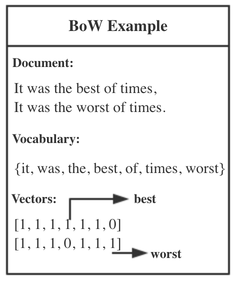
Figure 1. BoW Example
The problem is, if the vocabulary is getting too large, then the vector may become too sparse (containing too many 0s), due to limited words within each single sentence. One solution is to substitute each word (token) with N-gram. Taking bigram as an example, the first sentence will be tranformed into: {it was, was the, the best, best of, of times}
Part of Speech, POS & Chunking
Simply transforming text into numbers by counting the occurence is not strong enough to overcome text ambiguity. For example, ‘bear’ can work both as a noun or verb, but this difference can’t be identified by BoW. Part of speech (POS) tagging can classify each word into different groups, e.g. nouns, pronouns, adjectives, verbs, adverbs, prepositions, conjunctions and interjections.POS tells each word’s property, but actually word usually function in groups. Chunking solves this by taking POS tagging results as input, then output a set of chunks, which extract related words as phrases, like noun phrase, verb phrase.
Word Embedding
No matter how BOW or POS, chunking are designed to help finding a proper way to represent text in numeric format, they all have certain limitations. From my point of view, BOW is kind like tf-idf, a count-based method, despite of that td-idf tells word frequency, BOW only shows word existence. Both of them can’t point out whether certain words are closer than others. In this sense, chunking works slightly better than POS, as it shows phrases. But on one hand chunking can’t indicate to what extent they are close to the others, on the other hand, it only recognize common phrases. While for embeddings, e.g. CBOW, skip-gram, these two can identify word closeness based on the given text (its context, to be more specific). So even if uncommon or new phrase shows up in the text, its closeness can be recognized. BTW, word2vec is a very popular word embedding tool provided by Google. The model used in this tool is CBOW & skip-gram. Don't get confused.
CBOW & Skip-gram have been firstly proposed by Tomas Mikolov in 2013. These embedding methods enable to represent words in a denser-dimension space, and can group similar words. In the following part, I will talk about the principles behind these models and explain why they can caculate similarity among words.
CBOW & Skip-gram Similarity:
- Composition: Both CBOW and skip-gram models divide the text into 2 groups: target word and context (the size of the context depends on the size of the sliding window you set. Suppose the window size is 2, so the context would be 2 words on the left side of the target and 2 word on the right side, Context size: C, window size: N, C <= 2*N).
- Input: Words need to be firstly changed into one-hot encoding to pass onto the model. (Previously I got confused here, one-hot is very similar to BoW, but why CBOW can recognize word closeness, BoW can’t. Take yr time, I will explain it later.)
- 1st transformation: a V*N matrix W, V is the vocabulary size(not context’s), N is a arbitrary number which defines the size of the embedding space. Multiply one-hot word vector with W, get the vector changed into a size N embedding vector.
- 2nd transformation: a N*V matrix W’, multiply hidden layer vector with W’, get a size-V vector.
- Before generating output: softmax. (This part is kinda like logit function in Logistic regression. But LR aims to make its output value within [0,1], softmax ensures the sum of each element in the size-V vector equal to 1, so the element with highest probability would most likely be the target word)
- Updation: through backpropagation, update the parameters to adjust the output.(After all, the initial W & W’ are randomly generated)
CBOW & Skip-gram Difference:
- CBOW predicts which word would be the target word given context, while skip-gram works in an opposite way.
- CBOW: the multiplication of each context word one-hot vector with W need to be averaged before pass onto the hidden layer.
The best way to explain something is to show the principle with examples, so I will use one example to go through these two models’ working process.
- The corpus is: I drink coffee everyday.
- Target: coffee
- Window Size: 2
- Context: {I, drink, everyday}
as the corpus only contains 4 words, this size-2 window happens to include all the corpus. In the real world problem, the corpus size is usually much larger.
Continuous Bag of Words, CBOW

Figure 2. CBOW Framework with Example

Skip-gram, SG
The workflow of SG resembles CBOW’s process. Get one-hot encoding of target, multiplied by W to form the hidden layer, then multiplied by W’, generate C intermediate vectors for each context word. Then, same as CBOW, calculate probability by using softmax.
Attention these C intermediate vectors are generated by the same hidden vector and W’, meaning they are exactly the same. So how can SG make predictions on multiple context words? I will explain it in the parameter updation part.
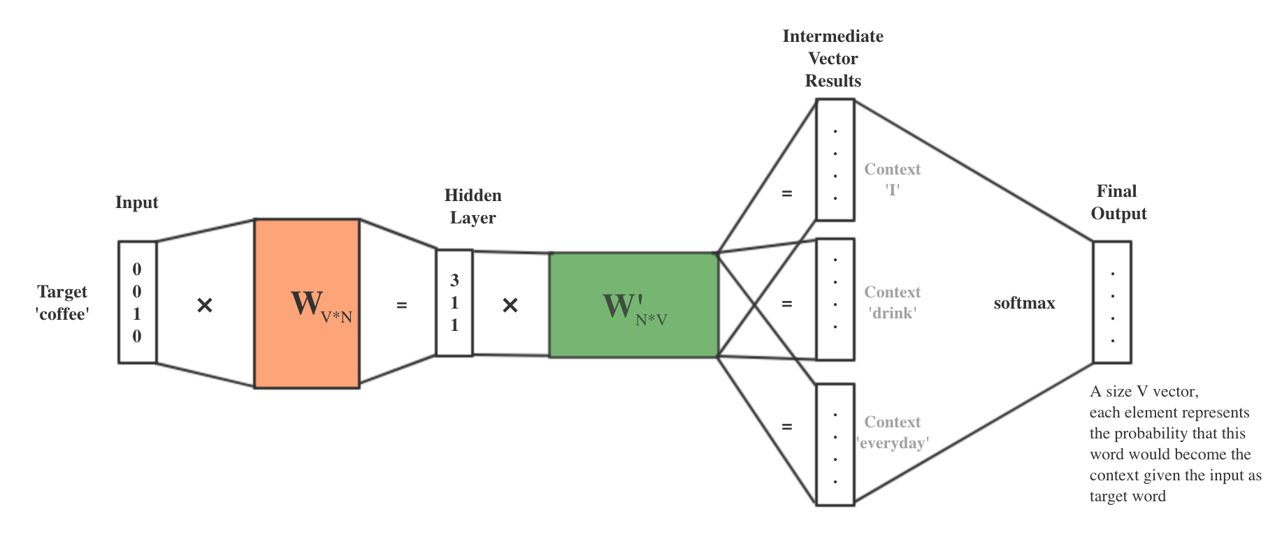
Figure 3. Skip-gram
CBOW & SG Model Parameter Updation Process
In the training process, each iteration contains two main stage:
- Forward propagation: using input word vector and random W, W’ calculating all the way to get the final probability output
- Backward propagation: evaluating the distance between your prediction and the true value, to adjust W’ and W(To be more specific, it’s about updating the correspoding column of W’ and row of W, based on the input word).
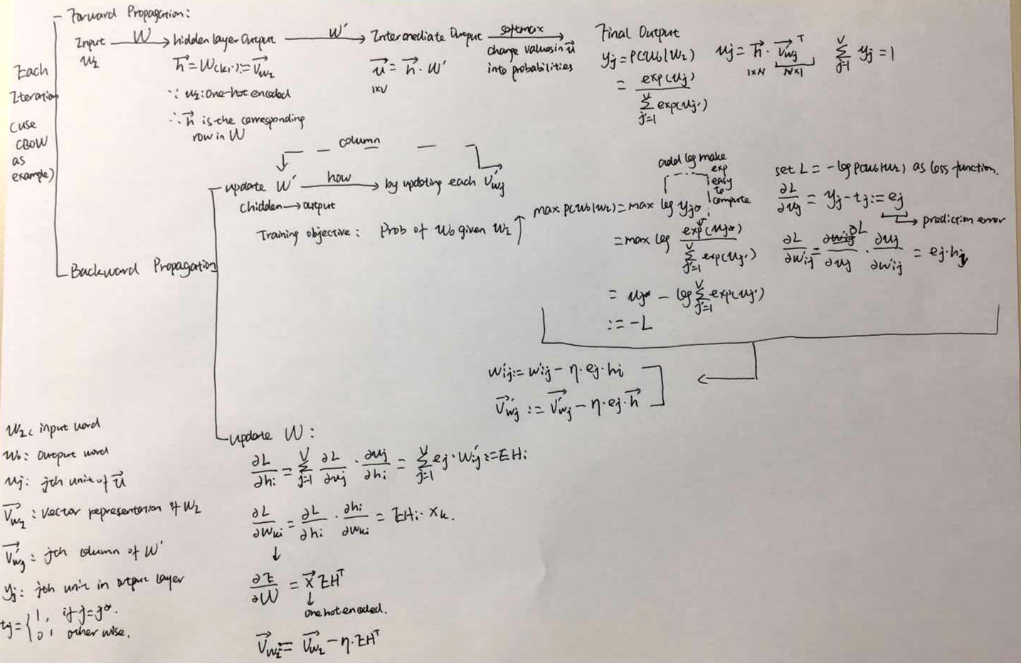
Figure 4. Updation (CBOW as example)
Answer to: how SG make predictions on multiple context words using the same . This is because different context word is shown at different index of
. Then through backward propagation, evaluating the error between the real context word and the prediction, the corresponding column of W’ will be updated to decrease the error. Finally, we can get different probabilities of different context words given the target word.

Figure 5. SG W’ Updation
Computational Efficiency: CBOW & SG Model Optimization
About softmax function, in the denominator section, it shows all the V words need to be computed in each iteration. So if the vocabulary is very large, then it’s too time-consuming to complete the whole process.
Hierarchical Softmax: one way is to utilize the property of binary tree: vocabulary is represented as leaf node, probability is calculated by using conditional probability(path: from root to leaf). Negative Sampling: The other way is to sample a sub-group of the vocabulary. The sub-group is composed of the ground truth word(positive sample) and a subset(negative sample), which is sampled based on a probabilistic distribution. Details are shown in [5], section 3.1 & 3.2.
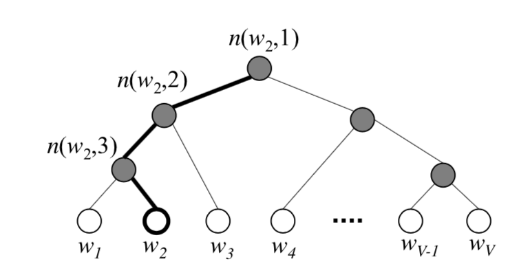
Figure 6. Hierarchical Softmax (Source: [5])
Answer to: using one-hot ecoding vector as input, multiplying by random generated W, W’, how can SG/CBOW calculate word similarity? From my point of view, this similarity can be defined in many degrees. 1. word closeness: some words are more close to each other in the text. This is adjusted by measuring the distance between your prediction and the ground truth word. Then, through updating W’, W, the probability of the word which is actually close to the target will be increased. Meanwhile, the probabilities of other unrelated ones will be decreased. 2. counterpart: (it is stated in [3] that vector(‘King’) - vector(‘Man’) + vector(‘Woman’) is close to vector(‘Queen’)). Because these counterparts tend to function as similar roles in text, work with similar group of words. Then it’s not hard to imagine there would be connections among their corresponding vectors.
GloVe
TBA..
Reference
[1]. https://en.wikipedia.org/wiki/Bag-of-words_model
[2]. https://medium.freecodecamp.org/an-introduction-to-part-of-speech-tagging-and-the-hidden-markov-model-953d45338f24
[3]. Tomas Mikolov, Kai Chen et al. Efficient Estimation of Word Representations in Vector Space
[4]. https://lilianweng.github.io/lil-log/2017/10/15/learning-word-embedding.html
[5]. Xin Rong. word2vec Parameter Learning Explained
[6]. Tomas Mikolov, et al. Distributed Representations of Words and Phrases and their Compositionality
[7]. CS224D: Deep Learning for NLP Lecture Notes: Part 1
[8]. https://iksinc.online/tag/skip-gram-model/
[9]. http://mccormickml.com/2016/04/19/word2vec-tutorial-the-skip-gram-model/
[10]. https://medium.com/district-data-labs/forward-propagation-building-a-skip-gram-net-from-the-ground-up-9578814b221
[11]. http://mccormickml.com/assets/word2vec/Alex_Minnaar_Word2Vec_Tutorial_Part_I_The_Skip-Gram_Model.pdf

Leave a Comment