Introduction

Finally, I’m writing something about neural network. I will start with the branch I’m most familiar with, the sequential neural network. In this post, I won’t talk about the forward/ backword propogation, as there are plenty of excellent blogs and online courses. My motivation is to give clear comparison between RNN, LSTM and GRU. Because I find it’s very important to bare in mind the structural differences and the cause and effect between model structure and function of these models. These knowledge help me understand why certain type of model works well on certain kinds of problems. Then when working on real world problems(e.g. time series, name entity recognition), I become more confident in choosing the most appropriate model.

RNN and Traditional ANN

No matter how deep or complex a neural network is, it is typically composed of 3 parts: an input layer, several hidden layers(1 or more) and one output layer. Within each layer, it tries to transform the input based on certain function(softmax, relu, logit) and selectively passes(dropout) the data onto the next layer. So, why NN is so powerful? In my opinion, the key is about data representation. With each layer’s transformation, ANN enables data to be represented in a more and more appropriate way. Then, useful information can be more easily to be extracted out. The left section in Figure 1, shows a three layer feed forward NN. Every node(except the output layer) in the network has been connected to all the nodes in the direct following layer. No connections are made within a single layer, meaning all nodes from one layer are independent.

For sequential NN, e.g. RNN, connections are existed both within layers and among layers(to be specific: the layer refers to the hidden layer). So why links within layers are needed? Because such links support information to be passed from node to node within layers. Then, why do we need to pass information sequentially in the same layer? Because when working on senarios, like language translation, context info is extremely important for the final translation. For example: ‘Patient A denied that he had diabetes problems.’ A feed forward NN would pass each word into a unit, and process the word independently from one layer to another. So the final output may be identified the patient had diabetes.

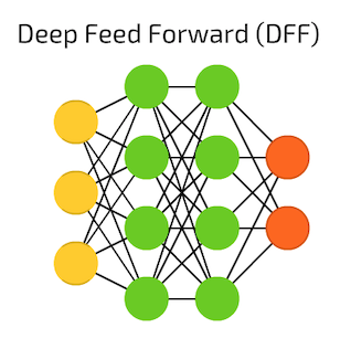
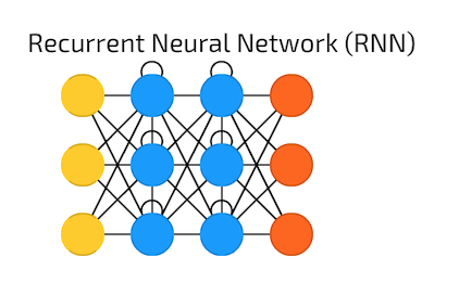
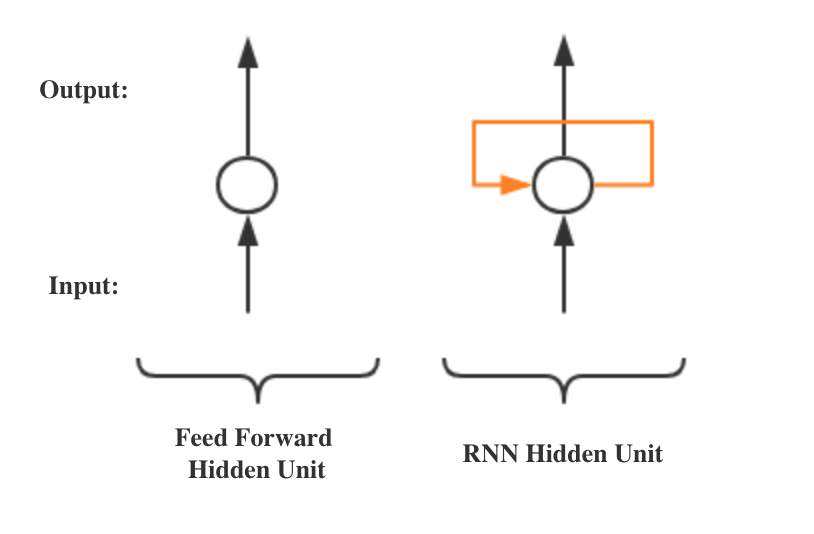
Figure 1. Deep Feed Forward NN and RNN _{Left & Middle Figure Source: Fjodor van Veen - asimovinstitute.org}

The intrinsic property of RNN is its hidden unit can capture previous info as memories, and this can be implemented by adding a loop to the original hidden unit(Shown in Figure 1. the bottom half). More details are shown in the left part in Figure 2. Memories of previous info would be passed through the loop in that graph, and the black sqaure indicates one time step delay interaction. The other way is to unfolding the operation by using multiple copies of a single unit, and the number of these copied units equals to the size of the input sequence. The first one is very succinct, while the second one allows the model use same transition functions and share parameters at every time step, which decreases the # of parameters a model need to learn.

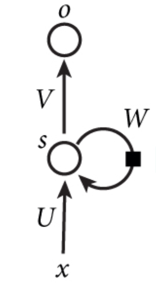
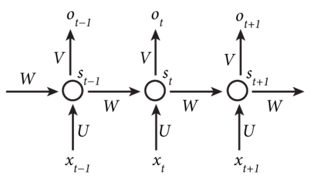
Figure 2. Folded and Unfolded RNN Hidden Unit Structure _{Source: Nature}

RNN Application Scenarios

So what is RNN capable of? What kind of scenarios can RNN be applied to? The answer is any scenes which are in great need of context information, e.g. NLP and Time Series tasks. To be more specific, the detailed structures of RNN can be customerized into different types, according to each task’s input and output requirements. For example, to summarize the content shown in a single image, a one-to-many structure would be a proper answer. For language translation, each word input needs to be translated. So the optimal structure would be many-to-many.

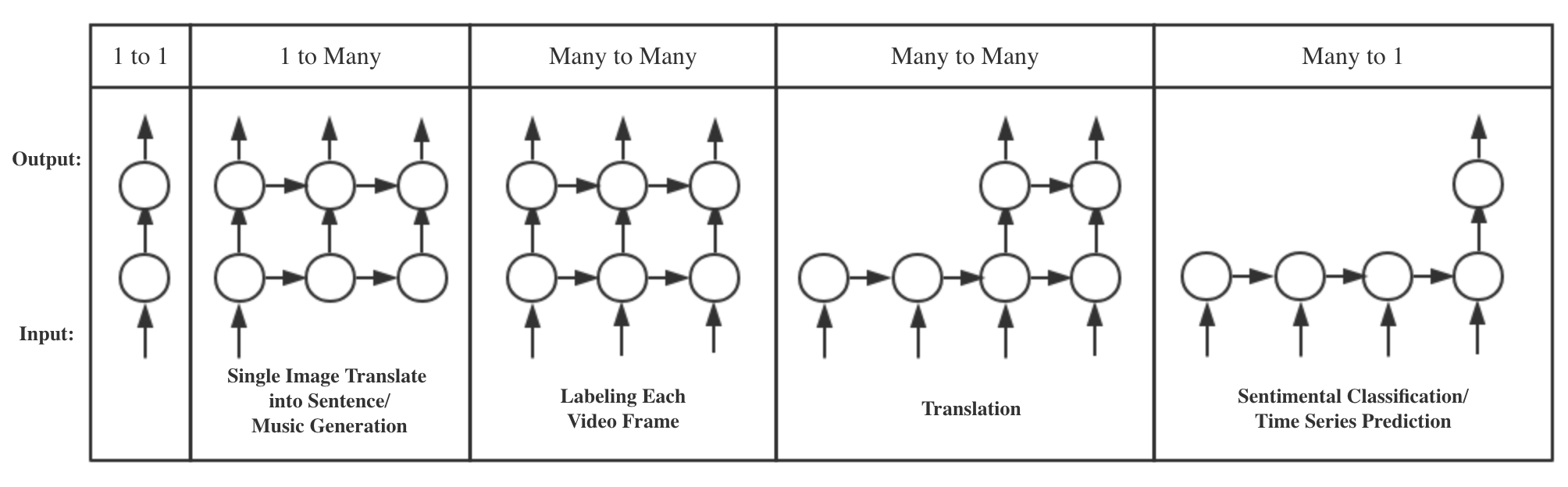
Figure 3. Different Types of RNN and Related Application Scenarios

Long Short Term Mememory Neural Network, LSTM

To fix this, LSTM has been invented. Compared to RNN, three switching gates have been introduced to control the flow of all info passed through the neuron unit. To clearly explain why LSTM can overcome this long term dependency problem, the best solution is to take a close look at its hidden unit structure.

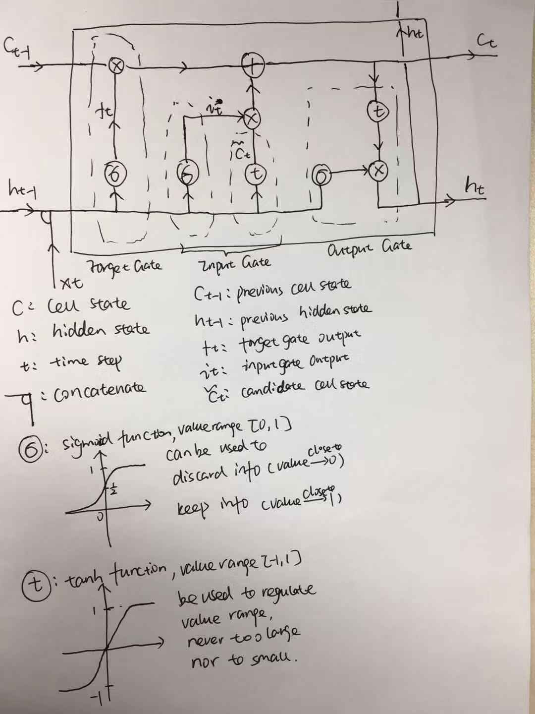
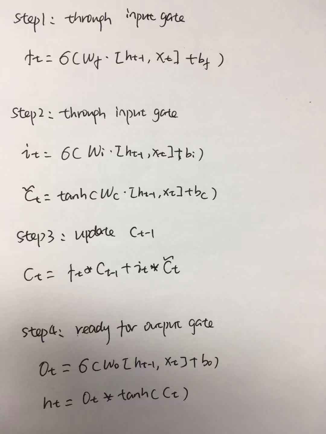
Figure 4. LSTM Hidden Unit Structure _{Please forgive my terrible handwriting}

Forget Gate: decides which part to be discarded from the previous cell state.

Input Gate: what new info will be added, to update the cell state, and limit the input value range.

Output Gate: what info will be kept to the next hidden state, and limit the output value range.

More details about LSTM, please see a marvelous post written by Christopher Olah. Here I will talk about how LSTM enables longer dependency compared to RNN. LSTM keeps two main flows carrying the info through all hidden units, instead of one. One flow would be processed through multiple nonlinear functions(sigmoid, tanh) for removing or keeping info. While the other will be only processed by simple linear operations, which is less likely to be lost. (The two horizontal lines in the left part of Figure 4 represent the two flows, carrying cell state info and hidden state info.)

Gated Recurrent Unit, GRU

There are several LSTM variants, containing various different computational components(e.g. peephole, full gate… details see in [6]), offering different roles and utilities. Here I’ll talk about a very famous variant, the Gated Recurrent Unit Neural Network.

GRU has removed the seperate cell state flow, and keeps only two gates: reset gate and update gate. The reset gate functions as the forget gate in LSTM, throwing away past info. The update gate decides what to throw from previous hidden state and what to keep in the candidate hidden state. Details shown in the following Figure.

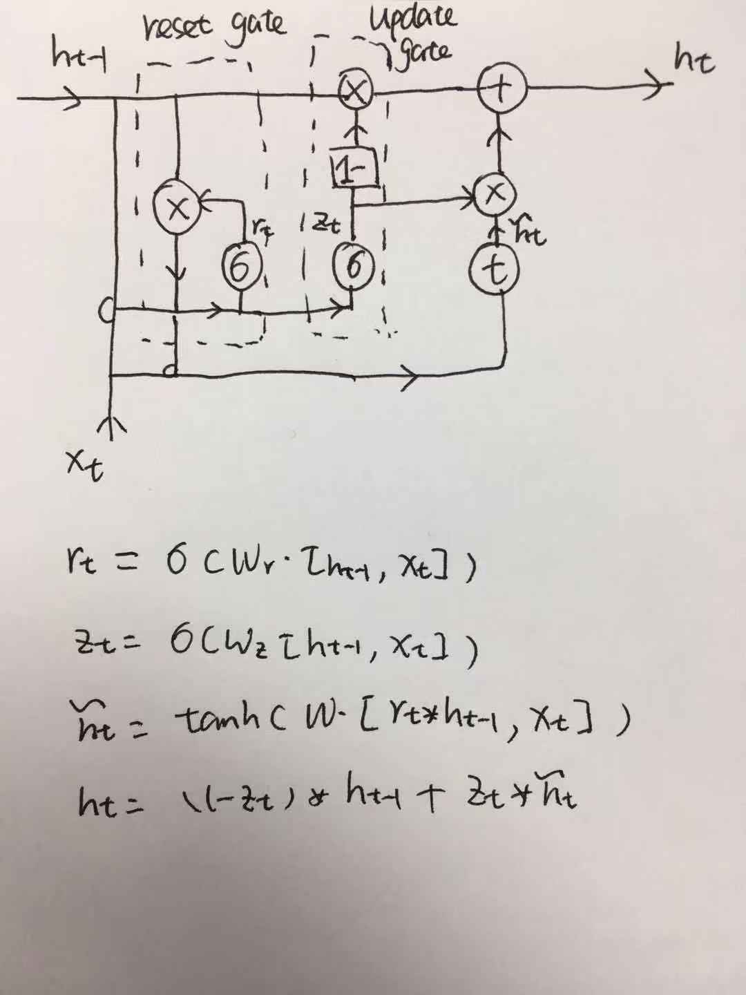
Figure 4. GRU Hidden Unit Structure

Though there is no seperate cell state flow in GRU, in my opinion, the top horizontal line carrying the hidden state info works similarly as the top cell state line in LSTM. Because only simple linear functions have been operated on this top line in GRU. Another difference between LSTM and GRU is GRU doesn’t control its input and output value range(no tanh function to control the range). About LSTM and GRU, which one is better? It’s hard to tell, after all them work in a very similar way. Maybe GRU runs faster to converge, due to less operations. I think the answer depends on the specific situation where these models have been performed.

Reference

[1].http://www.wildml.com/2015/09/recurrent-neural-networks-tutorial-part-1-introduction-to-rnns/

[2].https://colah.github.io/posts/2015-09-NN-Types-FP/

[3].https://en.wikipedia.org/wiki/Recurrent_neural_network

[4].https://colah.github.io/posts/2015-08-Understanding-LSTMs/

[5].Yoshua, B. Patrice, S. Learning Long-Term Dependencies with Gradient Descent is Difficult. IEEE TRANSACTIONS ON NEURAL NETWORKS 5(1994)

[6].Klaus, G. Rupesh, K. S. LSTM: A Search Space Odyssey. TRANSACTIONS ON NEURAL NETWORKS AND LEARNING SYSTEMS.

[7].Junyoung, C. Caglar, G. Empirical Evaluation of Gated Recurrent Neural Networks on Sequence Modeling.

[8].https://towardsdatascience.com/illustrated-guide-to-lstms-and-gru-s-a-step-by-step-explanation-44e9eb85bf21