
Tree Series 2: GBDT, Lightgbm, XGBoost, Catboost
Published:
Introduction
Both bagging and boosting are designed to ensemble weak estimators into a stronger one, the difference is: bagging is ensembled by parallel order to decrease variance, boosting is to learn mistakes made in previous round, and try to correct them in new rounds, that means a sequential order. GBDT belongs to the boosting family, with a various of siblings, e.g. adaboost, lightgbm, xgboost, catboost. In this post, I will mainly explain the principles of GBDT, lightgbm, xgboost and catboost, make comparisons and elaborate how to do fine-tuning on these models.
Gradient Boosting
Beforing elaborate the details, I will leave you 10 minutes to think about a few quick questions of Boosting, which will help you get clear with the procedures of this model. The key of boosting is sequentially learn the “lessons” made in previous round, so:
1. How to combine previous learners’ results with this round?
2. In what form to represent and add these previous results?
3. GB stands for gradient boosting, what’s gradient for in this algorithm?
Ready to go?
Gradient Boosting Machine learns the errors made in previous rounds, and tries to correct them. These errors are represented as residuals, to be more precise, it works on fitting the gradient of the residuals. That’s why it’s called gradient boosting.
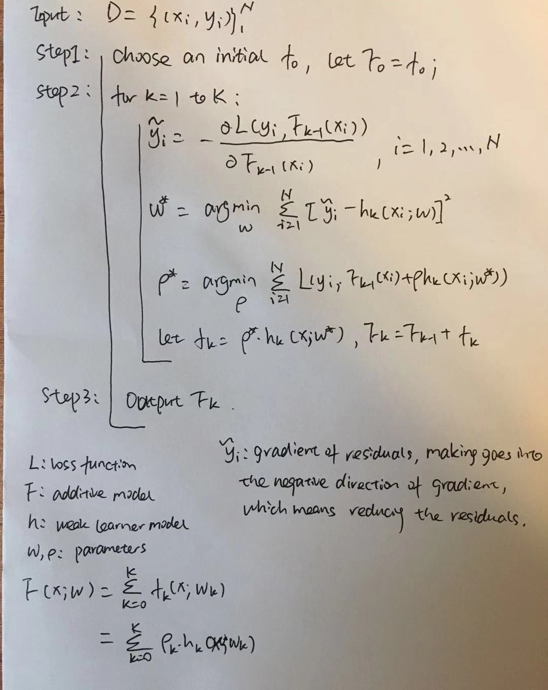
Figure 1. Gradient Boosting Machine Algorithm
Please forgive my twisted handwriting, writing down the algorithm by hand indeed helps me memorizing the details. In a nutshell, in the kth iteration, the algorithm tries to fit a new single learner hk into the last residuals. Shown in Figure 1, it minimizes the mean squared error of the residual and hk by finding the optimal w* . Then, add hk multiply a parameter ρ to Fk-1 to form Fk.
Quick question: why ρ is needed? why not directly add hk to F?
ρ can be viewed as a learning rate(learning step), it’s a strategy for avoiding overfitting. By adding a parameter, which is less than 1, though the learning speed will be slowed down, it guarantees the importance of each hk won’t become too much. Usually, a penalty Ω on tree complexity(a regularization method) will be also added to inhibit overfitting. I will summarize all the strategies for overfitting later.
GBDT
GBDT has some variation from GBM, e.g. hk is referred to DT in GBDT, Fk is the ensemble of DTs, residual equals to yi minus Fk-1, the searching space is J non-overlapping regions, {Rj}.
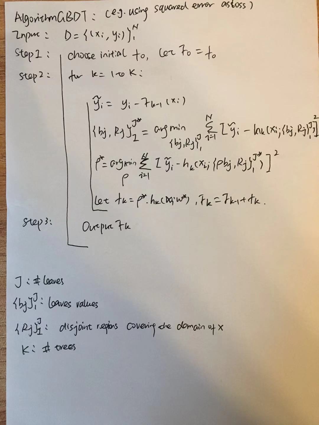
Figure 2. GBDT Algorithm
Table 1. Tree Constraints for overfitting
| Constraints | How & Why | Degree of Control |
|---|---|---|
| # trees | the more the better, as it averages the variance | relatively slow to decrease overfitting |
| Max depth | shallow trees have less chance to overfit, block bias splitting towards certain direction for each tree | relatively strong influencer |
| learning_rate: α | undermine the influence of each newly added tree, because the value of α is below 1 | relatively strong influencer |
| # leaves | set maximum limitation, there will be less split, means controlling tree complexity | |
| # instances per split | if a node’s # instances is less than certain threshold, or will be less than that number after split, then forbid this splitting, reason: same as above | |
| minimum loss improvement | if improvement < certain threshold, then forbid this splitting: reason: same as above |
In Table 1, I have listed the methods which could be used for controlling overfitting. These methods can be divided into 2 groups: one is limit the number of trees, the other is limit the complexity of each single tree. There are some other controlling methods, e.g. sampling, sub-sampling, I will included them later in the section about parameter tuning for specific tree models.
Finding Best Splitting
We know the best splitting comes with the point which maximize the loss function, but how to find the point? Let me explain this in a reversed way: the searching space for best split is limited, which is a set of proposed splits, and there are two ways to find the proposed split sets, one is exact greedy searching, the other is approximate algorithm.

Figure 3. Find Best Splits
As you can see from Figure 4, exact greedy algorithm goes through all the values in that feature for finding the split, it has an inner loop and an outer loop, so the time complexity would be O(# unique I * m). In order to make this algorithm less time-consuming, the values need to be firstly sorted. which is firstly sort all the values of that feature, then calculate the loss reduction for each value. For approximate method, it utilize percentile of that feature’s distribution as proposed points, then cut continuous feature into buckets based on these points, aggregate the statistics, and find the best point according to these information. The time complexity has been reduced to O(m). This algorithm has 2 branches, one is coming up with the proposals at the initial tree construction time, and use these proposals through the whole process. The other is calculate new proposals after each splits. It’s not hard to see the first one is more efficient, as it doesn’t to calculate proposals all the time. But the other would be more accurate for finding the point, so it’s better for growing deeper trees.

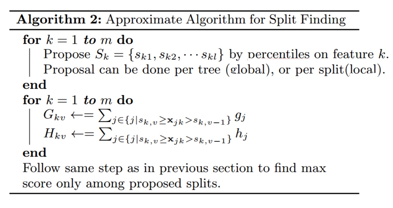
Figure 4. Splitting Finding Algorithm
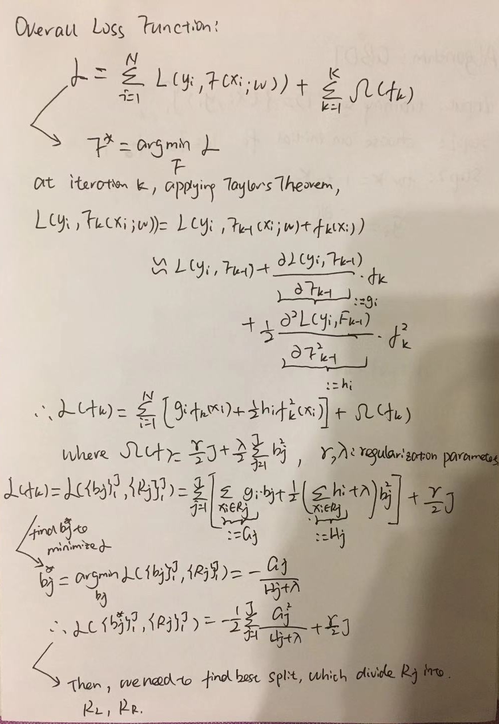
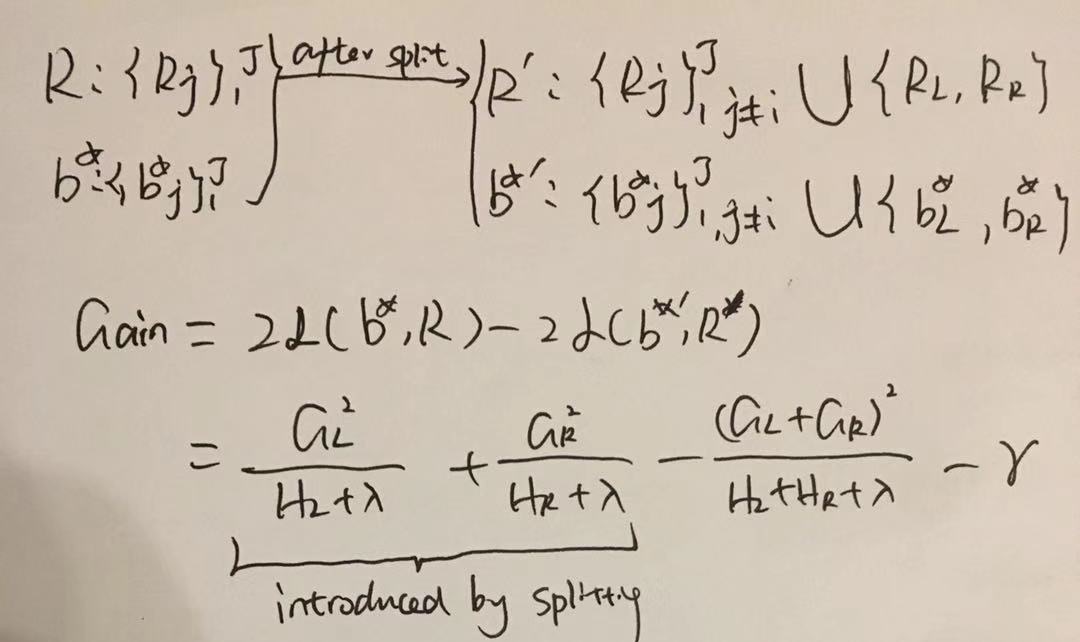
Figure 5. Approximate Algorithm
With all these knowledge and fomula in mind, then it’s much easier for you to understand the difference and improvement of Lightgbm, XGBoost, and Catboost compared to each other and GBDT.
XGBoost
We all know or have heard of XGBoost is extremely efficient, that’s why it becomes the most popular tools for Kaggle competition. But do you know why XGB can work so powerful and fast? `Pre-knowledge:
- disk: usually referred to hard drive. In order to process the data stored on disk, the CPU need to assign a thread to find the data from the disk, then fetch it into memory. Meanwhile, when searching on the disk, a head need to move across the disk to find the data. It is very time-consuming for all above processes.
- memory: e.g. RAM: random access memory(another version is ROM), no physical movement is needed for memory. ` 1. Reduce time by redesigning data access & storage
The most time-consuming part in tree learning is to sort the feature values. In order to reduce the time, XGB applies column block and cache-aware access strategies, which greatly reduces the data accessing time.
1.1 Column Block
XGB stores the data in a compressed column format in in-memory units, which called block. The feature values will be sorted only once before training, instead of doing sorting in each split finding iterations.
1.1.1 For exact greedy algorithm:
- the entire data is stored in a single block,
- one scan through the block can get all the statistics of the proposed points.
1.1.2 For approximate algorithm:
- data subset of rows stored in multiple blocks, instance indices are stored in blocks too,
- blocks can be distributed over machine, or even stored on disk,
- enables a linear scan over the sorted columns, and the statistics collecting for each feature can be implemented parallelized,
- block also supports column subsample, which I will talk later.
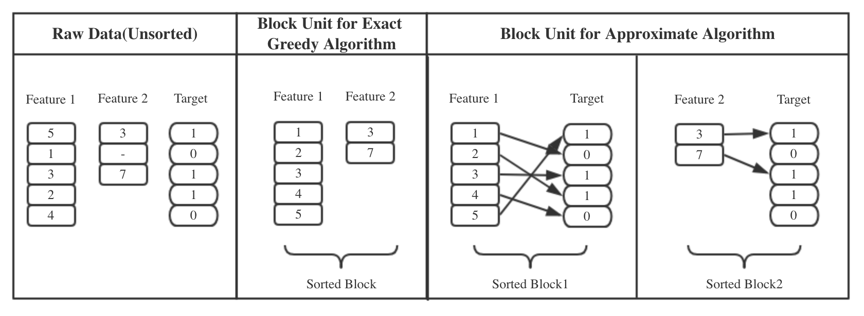
Figure 6. Example for Block Parallel
1.2 Cache-aware Access
The model fetches statistical info by instance row index. However, as the instances are sorted by values, the access to these row indices will be non-continuous. When these statitics doesn’t fit into CPU cache, the accessing speed will be slowed down.
1.2.1 For exact greedy algorithm:
- Using a thread pre-fetches instances from non-continuous memory into a continuous buffer(in-memory & physical continuous),
- then perform gradient statistics accumulation in the continuous buffer.
1.2.2 For approximate algorithm:
- still use block for pre-fetching, but need to be careful about the size, if too large, the calculated gradient statistics can’t fit into CPU cache, otherwise, can’t store enough data, not efficient for parallelization.
1.3 Out-of-core Block
It’s mentioned above, blocks can be distributed in disk, which will increase the time in doing disk I/O reading. To solve this, XGB will authorize an independent thread to pre-fetch the block into buffer, which will enable concurrence between computation and disk reading. Besides, XGB has also applies two other tricks to improve this out-of-core computation.
1.3.1 Block Compression: data will be compressed by columns in block, and decompress on-the-fly when loading into memory. This method helps to reduce reading time, as size of the compressed block is definitely smaller than the original one.
1.3.2 Block Sharding: store the data subset distributedly in multiple disks, assign each disk a pre-fetcher thread, Then, the training thread can altervatively reads the data. (Referenced from [6], this part is a little confusing to me. At first, I thought the improvement made by block sharding is to enable multiple threads read these distributed disks at the same time, which means parallelization. But later, I realized it might be a different case: e.g. the sharding strategy stores subset A, subset B on different disks. When it comes with the case that only B is needed, so the thread can directly touch the disk where B is on. Otherwise, A and B stored in one disk, the thread need to pass through the whole data to find B. Please correct me, if I’m wrong.)
2. Reduce time by improving the algorithm: enable automatic sparse data handling
Sparse data is very common in both classfication and regression problems, when doing split finding, XGB offers a new option to be aware of these sparse data. Shown in Figure 7, when doing value sorting, only non-missing entries will be accessed. Such strategy helps to reduce the time cost for sorting. XGB also adds a default direction in each node. when coming across a missing value, the entry will be classified into the default direction.
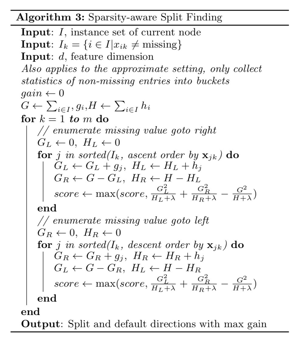
Figure 7. Sparsity-aware Split Finding Algorithm
Lightgbm
XGB provides both exact split searching(enumerate all instances) and approximate searching(histgram-based), while lightgbm mainly works on the second one, and maintains relatively accurate results at the same time. In this sense, lightgbm is typically faster than XGB. To achieve the above goal, lightgbm proposes 2 techniques: Gradient-based One-side Sampling(GOSS) and Exclusive Feature Bundling(EFB).
1.1 GOSS: reduce data size by rows
Typically, instances with larger gradients will contribute more to information gain, compared to the ones with smaller gradients(e.g. think about a data set whose distribution is uniform). Thus, keeping all the instances with large gradients, while removing the smaller ones, such method seems to be a good choice. However, if we directly remove all the small gradient data, the distribution would be distorted, and the result accuracy would be lost too. So lightgbm keeps data with large gradients. So how to target at the large ones? It can be done: 1. using pre-defined threshold to select large gradients,
- or selecting top percentile. Lightgbm sets a sampling ratio a to select the top ones(need to calculate the gradients first, and use the absolute values).
And randomly drop the ones having small gradients, by using a ratio b. To compensate for data loss, lightgbm uses a constant to amplify the small gradient instances when calculating the information gain.

Figure 8. GOSS Algorithm
1.2 EFB: reduce data size by columns
EFB aims to eliminate uneffective sparse features,(which are usually mutually exclusive, e.g. one hot encoded feature sets), by bundling them into a single one. Algorithm 3 in the following figure shows how lightgbm find the features to bundle. It firstly builds a graph, using edges to represent total conflicts among features, then sort the features by the degree in the graph, based on these knowledge, assign the feature to its correponding bundles. Algorithm 3 is not fit for the data with too many features, so lightgbm improves this by using counting of non-zero values to substitute building the graph. algorithm 4 is about how to transform these features into one. The new feature will be represented in bins, and the key is to make sure the relation between each original feature and new feature bin. is 1 to 1. That’s how lightbgm can identify the original feature from these bundles.

Figure 9. EFB Algorithm
Catboost
Finally, here comes to the last model in this post, Catboost, a relative young sibling of all these ensemble trees. The first three letter ‘cat’ stands for category, because this model can directly handle discreet features, no matter it’s in numeric form, string or something else. That is users don’t need to transform categorical features into numbers before importing the data into catboost. So how is this section implemented in catboost?
1. How catboost deals with categorical features?
1.1 A common way is to substitute the feature value with averaged response value on the whole training set:
j: the instance index for the whole training set, k: the kth feature, which is a categorical, i: index of the instances which are from the same group in feature k, the denominator represents the count of feature K’s certain value shown in the whole training set.
The problem for above formula is if there is only one instance in the training set which belongs to the kth feature’s certain value, then the result is just this instance’s label value, which may cause overfitting. To solve this, catboost introduces random data permutation, two other parameters and calculate the averaged label on these random set instead of the whole training.
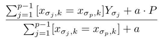
P: a prior value, a:(>0) weight of the prior. The prior helps to reduce the noise from low-frequency categories. For regression, prior is calculated by take average label value. For binary classification: prior equals the probability of encountering a positive class.
1.2 A simpler way implemented in catboost is to calculate the frequence of the categorical features, and use this frequence for substitution.
2. Feature Combination
Another improvement is automatic greedy feature combinations. The model will consider all combinations of the categorical features, but these combinations won’t be used for the first tree split. Catboost also enables combination of numerical and categorical features.
**Tips:** Users need to specify categorical features in catboost, or the model will either treat it as numeric by default.
3. Unbiased Gradient
The third improvement in catboost is calculating the gradient without bias. Typically, boosting tree models use the same data to estimate gradients and build model, which may cause overfitting. In catboost, it implements these two parts on different data. The basic idea is making random permutations on the training, then implement gradient estimation and tree building on different permutations.
Figure 10. EFB Algorithm
Reference
[1].Friedman, J. H. (February 1999). “Greedy Function Approximation: A Gradient Boosting Machine”.
[2].http://www.flickering.cn/machine_learning/2016/08/gbdt%E8%AF%A6%E8%A7%A3%E4%B8%8A-%E7%90%86%E8%AE%BA/
[3].https://en.wikipedia.org/wiki/Gradient_boosting
[4].Anna Veronika Dorogush, Vasily Ershov, Andrey Gulin “CatBoost: gradient boosting with categorical features support”. Workshop on ML Systems at NIPS 2017.
[5].Guolin Ke, Qi Meng, Thomas Finley, Taifeng Wang, Wei Chen, Weidong Ma, Qiwei Ye, Tie-Yan Liu. “LightGBM: A Highly Efficient Gradient Boosting Decision Tree”. Advances in Neural Information Processing Systems 30 (NIPS 2017), pp. 3149-3157.
[6].Tianqi Chen and Carlos Guestrin. XGBoost: A Scalable Tree Boosting System. In 22nd SIGKDD Conference on Knowledge Discovery and Data Mining, 2016

Leave a Comment