Clustering-DBSCAN

Disadvantages of Partitioning and Hierarchical Methods

Before introducing density clustering algorithm, I will first talk about the shortcomings of other clustering methods. Partitioning algorithm, such as k-means, it requires to declare k in the first step of clustering. Moreover, it has restrictions on the shape of clusters (convex shape), meaning it requires gaussian shape clusters.

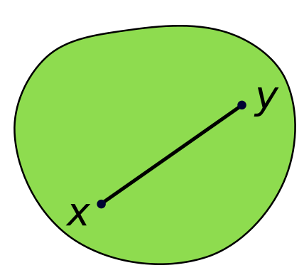
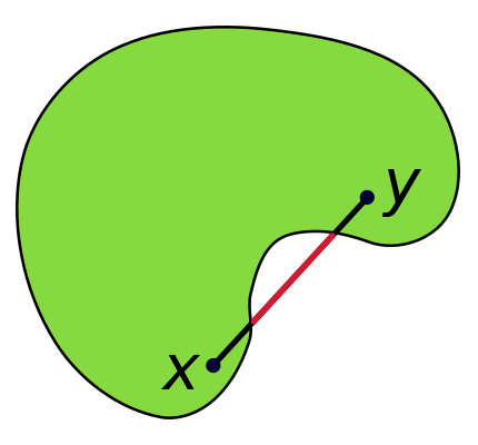
Figure 1. Convex Set and Non-convex Set

Example of K-means working on non-convex data: I have faked a banana shape dataset, and used kmeans with 2 clusters and 3 clusters to group the data. Shown in the Fig. 2, which will help you understand why kmeans works badly on non-convex data more easily.

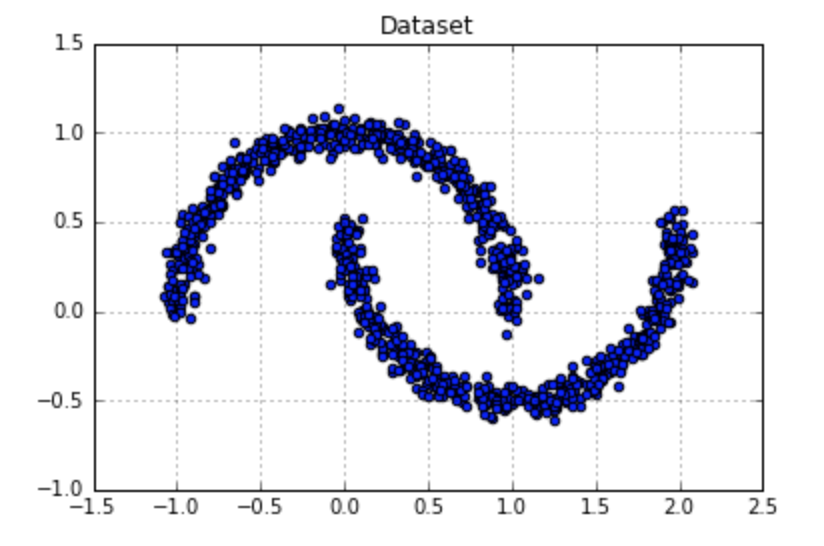
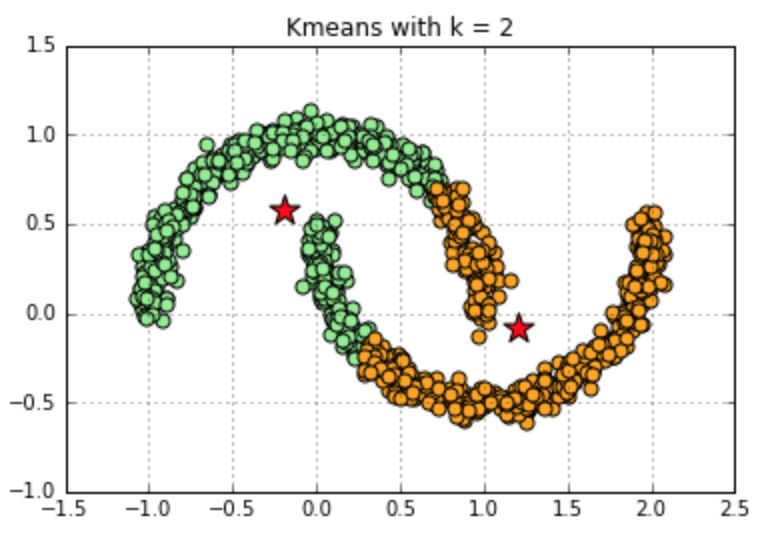
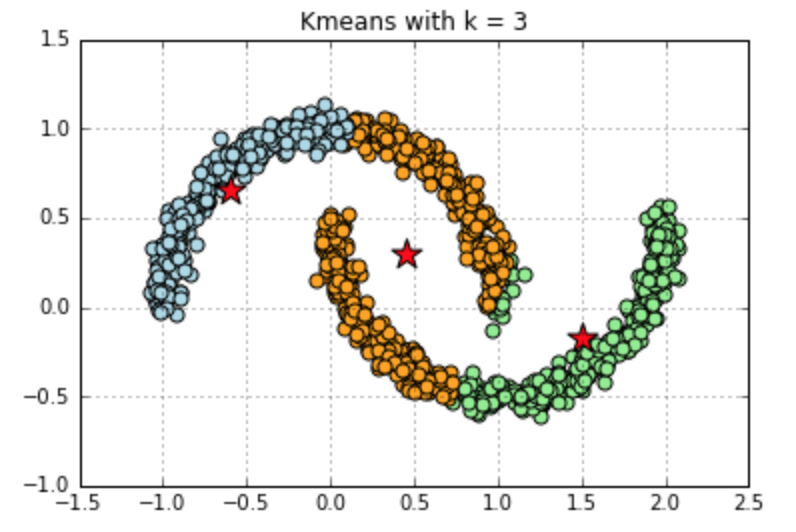
Figure 2. Kmeans with Non-convex Data

Hierarchical algorithm: it is hard to define termination conditions. For example, it is difficult to determine the value of D_min, which is small enough to seperate all clusters and large enough such that no clusters are being split. Here we use agglomerative clustering as example, results shown in Fig. 3.

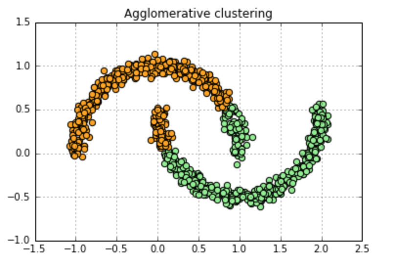
Figure 3. Agglomerative clustering

Compared to these 2 algorithms, DBSCAN (a density-based method) only has a minimal requirement of input, allows arbitrary cluster shape, resistant to noise and works efficiently on large dataset.

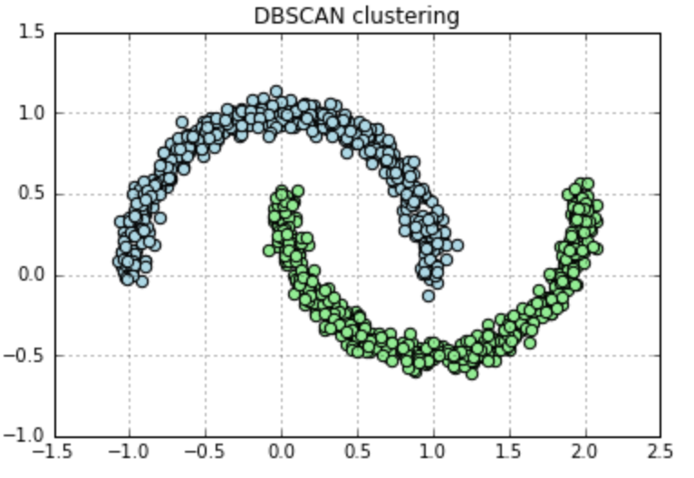
Figure 4. DBSCAN

Define Density

Since it’s a density-based problem, we need to know how to measure the density of points. I will introduce 2 important parameters and a few definitions. The Eps-neighborhood of a point p, known as N_Eps(p), is defined by N_Eps(p) = {q ∈ D | dist(p,q) ≤ Eps}

MinPts: a minimum number of points.

Core point: has at least MinPts neighbor points in an Eps ε of it.

Border point: is a point that has fewer neighbors than MinPts within ε , but lies within the ε radius of a core point.

Noise point: all other points that are neither core nor border points.

Directly density-reachable: p is directly density-reachable from q, if p ∈ N_Eps(q) and |N_Eps(q)| ≥ MinPts (core point condition).

Density-reachable: p is density-reachable from q, if there is a chain of points, p₁,…p_n, p₁ = p, p_n = q such that p_i+1 is directly density-reachable from p_i.

Density connected: p is density-reachable to q, if there is a point o that both p, q are density-reachable from o wrt. Eps and MinPts.

Cluster: Let D be a database of points. A cluster C is a non-empty subset of D satisfying the following conditions: 1) ∀ p, q: if p ∈ C and q is density-reachable from p wrt. Eps and MinPts, then q ∈ C. (Maximality) 2) ∀ p, q ∈ C: p is density-connected to q wrt. EPS and MinPts. (Connectivity)

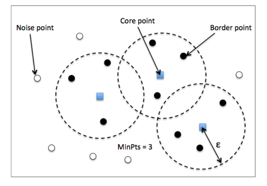
Figure 5. Different Types of Points

Algorithm

After get clear with the important definitions, let’s go into details of DBSCAN algorithm. The basic idea is clusters are dense areas in the data space, which have been seperated by regions of lower object density.

For each p ∈ D do
	if p is not yet classified then
		if p is a core-object then
			C = retrieve all density-reachable points from p wrt. Eps and MinPts
			make all objects in C as processed
			report C as a cluster
		else assign p to NOISE
		end if
End For

Determining Eps and MinPts

One common method is to make k distance plot, which calculates k distances of all points, and sort your results in decreasing order. Ideally, you will find a ‘knee’ in your plot. The objects on the left side of the ‘knee’ represents the border objects. By default, you can try to set MinPts as 2*Dimension-1 first. But you can also adjust this value to find better performance. Here is an example using k distance plot to find parameters for DBSCAN. From the 13-NN distance plot, I find a ‘knee’ at the distance of 0.3. Then, I applied DBSCAN by setting EPs = 0.3, MinPts = 13, and got the clusters as below.

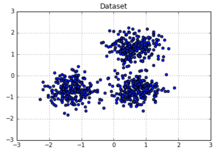
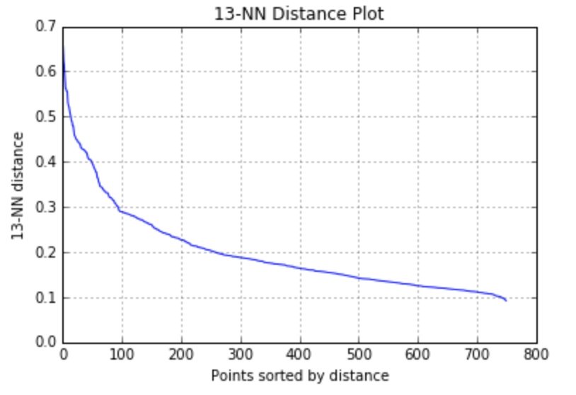
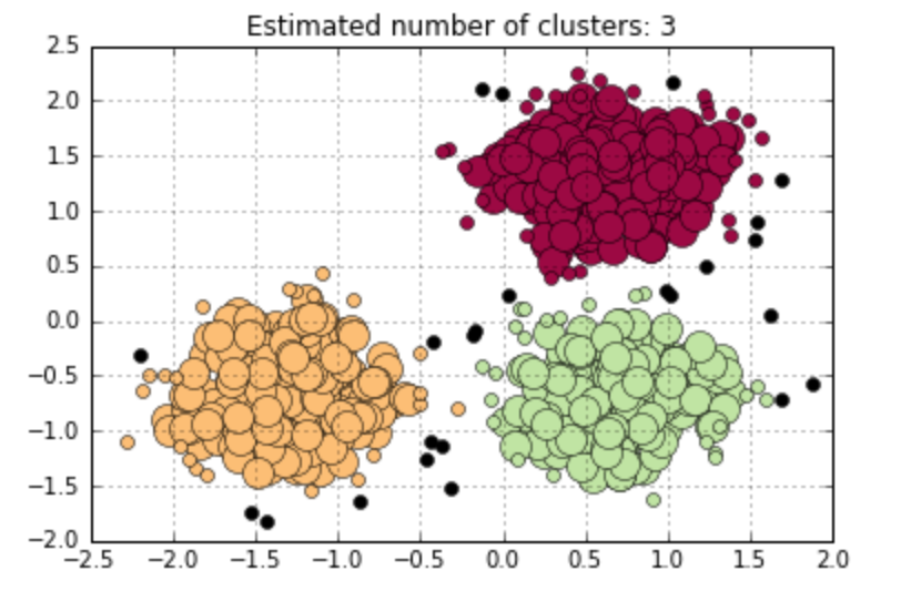
Figure 6. Utilizing k distance plot

But most of the time, I can’t find a very clear ‘knee’ from the distance plot. So I will select a set of parameter combinations, and then evaluate them from the cluster visualizations and coefficients, such as silhouette coefficient, homogeneity and so on.

When DBSCAN doesn’t work?

Advantage: based on previous analysis, we know DBSCAN requires less input information, the number of clusters are determined automatically, can identify noises and have no restrictions on cluster shapes.

It seems like a quite perfect clustering algorithm. However, it can’t work well on dataset with multiple densities. Let me use an example for illustration. You can notice two dense groups in the right upper corner and left bottom part, together with a less dense big group in the middle part. When I set eps at 1.1 with MinPts at 10, DBSCAN terribly group all the data into a whole. If I try to decrease eps value at 0.7, DBSCAN can identify the two dense groups I have mentioned before, but at the expense of dividing the middle scattered group into too many small clusters. This is very understandable. Because if you apply a very strict (Eps, MinPts) pair, the algorithm will work well on dense area, leaving loose area grouped into too many subsets. Otherwise, it is highly possible that DBSCAN can’t tell the dense area apart from the whole dataset.

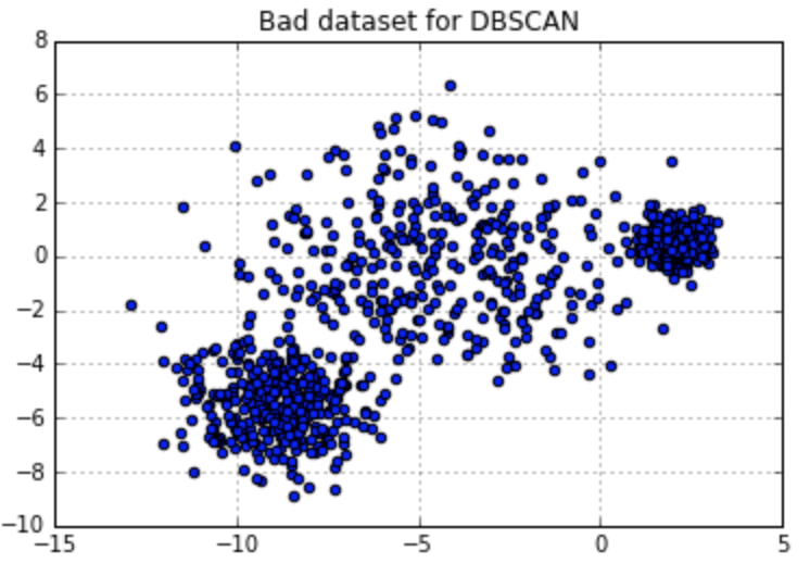
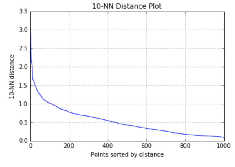
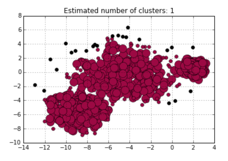
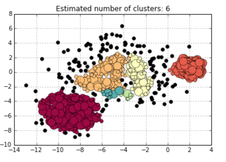
Figure 7. DBSCAN Works on Data with Various Densities

Reference

[1]. https://en.wikipedia.org/wiki/Convex_set

[2]. https://pafnuty.wordpress.com/2013/08/14/non-convex-sets-with-k-means-and-hierarchical-clustering/

[2]. Martin Ester et al. (1996). A Density-Based Algorithm for Discovering Clusters in Large Spatial Databases with Noise, Kdd 96(34), 226-231.