
Introduction of Reinforcement Learning, Part 1
Published:
Introduction
Recently, I have read some papers about Reinforcement Learning (RL). To me, it’s quite an interesting topic. But it’s also very complex, as it involves so many terms, definitions and methods. So I wrote this post to make an introductary overview of RL.
RL is mainly about through interacting with the environment sequentially, the agent will learn how to take actions to maximize an accumulative reward. It acts like an infant, who can’t speak yet. So he learns by observing the environment, making trials and getting responding results. If it’s a good behavior, he will know by getting reward. While bad ones will lead to punishment.
This concept is easy to understand. But before illustrating the core elements of RL, I’d like to stop here and ask a few questions. We’ve already got a lot of super powerful “learning”, like machine learning, sub-areas: supervised learning, unsupervised learning. What’s the relationship between RL and these existing ones? Why RL is still necessary? The answer is RL is also a sub-area in machine learning. You can see the differences in the table below.
| Supervised Learning | Unsupervised Learning | RL | |
|---|---|---|---|
| Input | labeled data | unlabeled data | initial state |
| Working Process | train on training set, look for model to optimize certain object function | look for model to gain insights into data | learn from environment in a sequential process, take actions, either being punished or rewarded, aiming to maximize reward, |
| Validation | validate on testing set | evaluate by reward function | |
| Application | regression, classification | clustering, segmentation, association | prediction, control |
Core Elements
A RL system contains 6 core elements: agent, environment, policy, reward signal, value function and model of the environment. In my opinion, the agent and environment is kind like entity, and the rest four elements are like attributes belong to entity.
On agent side: Policy helps agent map environment states to corresponding actions, which can be viewed as a set of responding behaviors in psychology. It can either be deterministic, a = π(s); or stochastic, π(a|s) = P[A=a| S=s]. Reward signal defines good/ bad events for agent. Thus, if the corresponding reward of an action is low, then the policy may be changed in the next step. Value function predicts future rewards.
On environment side: Model is optional in RL system, it could predict what environment will do next, including next reward and next state. Therefore, the agent can use it to do planning. While model-free RL can only acquire an optimal behavior by making interactions with environment through trial and error.
In general, the basic process of RL is from one state to another, the agent choose actions based on information (current state) of environment. This action will be emitted to change the state of environment. And the environment will in turn outputs a reward back to the agent.
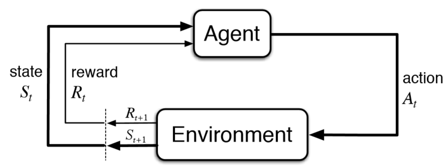
Figure 1. Agent & Environment Interactions
Markov Decision Process
A RL problem be defined as a Markov Decision Process (MDP). Because each state satisfies markov property, meaning the future state are independent of any previous states or actions. About the environment, it can be fully observable, or partially observable. When the agent partially observe the environment, meaning the observations received by the agent is dependent on the current state and the previous action, it becomes a partiarlly observable Markov Decision Process (POMDP).
Attention: POMDP is still MDP, as it can be converted into MDP.
A MDP can be represented as a 5-tuple (S, A, P, R, γ). S: set of states, A: set of actions. P: transition probability, R: reward function, γ: a discount factor, ranging from 0 to 1.
Why γ < 1: because it can prevent infinite accumulation of rewards in a non-episodic MDP, where there is no terminal state. While in an episodic MDP, the state will be reset after each episode of a certain length. If γ close to 0, it leads to short-sighted evaluation, otherwise, it will lead to far-sighted evaluation.
To solve the MDP problem, there are 2 fundamental methods: value-based and policy-based.
Value function includes state-value function and action-value function. The state-value function is about given policy π to select actions, then we can obtain: Vπ = E[ Gt | St = s] Of course, there be an optimal result: V* (s) = maxπVπ(s) Where, Gt denotes the total sum of discounted rewards from time t:
Gt = Rt+1 + γRt+2 + … = ∑k=0∞γk Rt+K+1
The action-value function denotes as being in state s and take action a, the expected reward will be: qπ(s,a) = E[ Gt| St = s, At = a], and the optimal q* means how good for an agent to take action a in state s. And the relationship between V* and q* is V* (s) = maxa q* (s,a)
To solve these equations, we can apply Bellman equation, which help to rewrite the value function in terms of the payoff from one initial state and its successors (immediate reward and discounted accumulative reward from successors). Let’s state-value function as an example:
Vπ = E[ Rt+1 + γRt+2 + … | St = s] = E[ Rt+1 + γGt+1 | St = s]
Value iteration begins with a random value function, then iteratively update new the q and V value function until reaching the optimal one (converges).
Policy iteration methods search for optimal policy π* to maximize the expected return. It contains two steps. Policy evaluation: given current policy, which is fixed, calculate values, iterate until values converge. Policy improvement: given fixed values, find optimal action using one-step look-ahead.
About value iterate, it need to calculate all actions in each iteration, which can be slow. Also, the policy may converge before the values. In every pass, it needs to update both values (explicitly) and policy (possibly implicitly). About policy iteration, it will conduct several passes to update utilities with fixed policy.
To be continued…
Reference
[1]. Sutton, R. S. & Barto, A. G. (1998) Reinforcement Learning: An Introduction. Cambridge, Mass.: MIT Press.
[2]. Leslie, P. K. (1996) Reinforcement learning: A survey. Journal of artificial intelligence research 4, 237-285
[3]. https://en.wikipedia.org/wiki/Bellman_equation
[4]. http://www.cs.ubc.ca/~murphyk/Bayes/pomdp.html
[5]. Si, J. (2004) Reinforcement Learning and Its Relationship to Supervised Learning. doi: 10.1002/9780470544785.ch2
[6]. Kai, A. (2017) A Brief Survey of Deep Reinforcement Learning. IEEE Signal Processing Magazine, 34(6), 26-38, arXiv:1406.2040
[7]. Yuxi Li. (2017) Deep Reinforcement Learning: An Overview. arXiv preprint arXiv:1701.07274
[8]. http://www.cs.ubc.ca/~murphyk/Bayes/pomdp.html
[9]. https://medium.com/@m.alzantot/deep-reinforcement-learning-demysitifed-episode-2-policy-iteration-value-iteration-and-q-978f9e89ddaa

Leave a Comment