SVM: Support Vector Machine

Published: May 21, 2016

The key of SVM is to find a hyperplane, which is built on some important instances (support vectors), to seperate data instances correctly. Here comes with a very contradictory process to construct the plane: the margin of the hyperplane is chosen to be the smallest distance between decision boundary and support vectors; at the same time the decision boundary need to be the one which the margin is maximized. This is because there can be many hyperplanes (Fig. 1) to seperate data correctly. Choosing the one which leads to the largest gap between both classes may be more resistant to any perturbation of the training data.

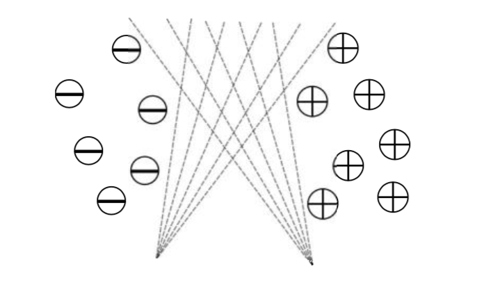
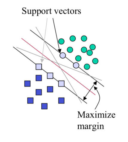
Figure 1. infinite hyperplanes and maximum margin

Functional Margin & geometric margin

Let’s take a two-class classification problem using linear models as the example.

y(x) = w^Tφ(x) + b

W: a weight vector; φ(x): input vector; b: bias; training set: N input vectors x₁,…, x_N, with corresponding target values t₁,…, t_N where t_n ∈{−1,1}; so the decision boundary can be represented as w^Tφ(x) + b = 0; for the 2 classes, one satisfies y(x_n) > 0, meaning t_n = 1; the other satisfies y(x_n) < 0, meaning t_n = -1, so that t_n*y(x_n) > 0. In this way, we define the functional margin as γ = t*(w^Tφ(x) + b), and we want to find the minimum functional margin over the whole training set.

$\hat{\gamma} = min \hat{\gamma_i} (i = 1,..., N)$ But when we multiply w, b, the value of functional margin will change too. So we introduce geometric margin, which represents the distance between a point to the hyperplane. ${\gamma} = \frac{1}{||w||}* \hat{\gamma}$

For the training set, ${\gamma} = min {\gamma_i}$

Maximum Margin Classifier

So the problem becomes:

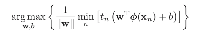
As we have mentioned before, if we change w → κw and b → κb, the distance from x_n to the decision boundary is unchanged. So we set this freedom to t_n (w^Tφ(x_n) + b)= 1; so all training set will meet the constraint: t_n (w^Tφ(x_n)+b) >= 1, n=1,…,N.

Then the problem can be changed into:

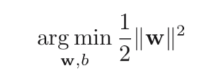
s.t. t_n (w^Tφ(x_n)+b) >= 1, n=1,…,N.

To make this constrained optimization problem much easier to solve, Lagrange Duality has been introduced. (a_n represents the Lagrange multiplier, a_n >= 0) This procedure can also help us to work on non-linear classification problem, by introducing a kernel function.

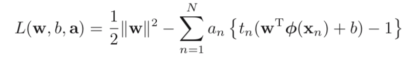
The problem becomes:

The dual problem is:

Details of this transformation is shown at the end of this blog.

Then, set the derivatives of L(w, b, a) with respect to w, b to 0, we get 2 conditions:

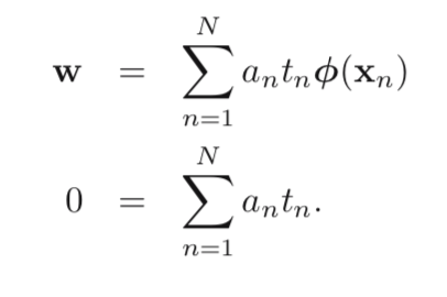
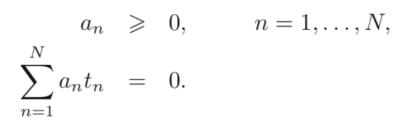
Put these 2 conditions back into previous formula:

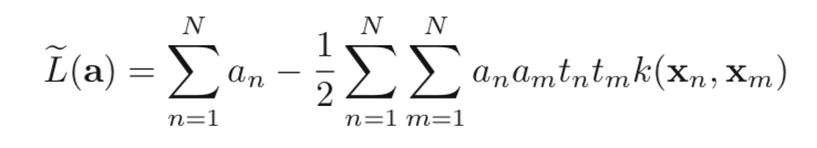
s.t.

Soft Margin: Introducing slack variable ξ_n to allow misclassified data: ξ_n = 0, represents data on the correct side of margin, or correctly classified; 0 < ξ_n <= 1, means data inside of margin, but on correct side of decision boundary; ξ_n > 1, denotes data on the wrong side of decision boundary. Thus, we want to minimize:

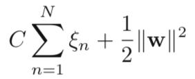
where C > 0, it controls the trade-off between the slack variable and the margin. Then, the Lagrangian formula is defined as:

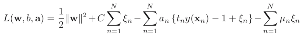
With KKT conditions:

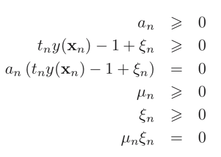
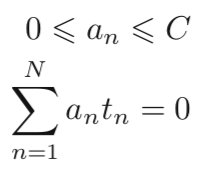
Again set the derivatives with respect to w, b, ξ_n to 0, then we get, and obtain the new form of Lagrangian, in which we maximize it with respect to a:

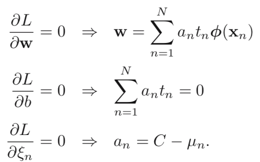
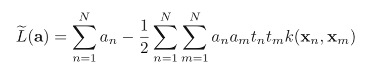
s.t.

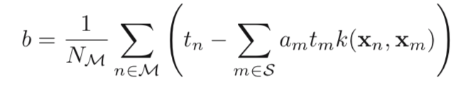
Then, we can obtain b by averaging:

Inner Product: In previous formula, k(x_n, x_m) can be viewed as the inner product of two vectors.

If x_n, x_m are parallel, there inner product is maximized.
If x_n, x_m are perpendicular, then their inner product is 0.

Let’s take a look back at the Lagrangian formula. Being perpendicular means two features are completely different, as there product is 0, it won’t influence the value of L. However, if they are parallel, meaning x_n, x_m, both features are completely alike. if 2 features predict the same class output, then a_na_mt_nt_mk(x_n, x_m) will be positive, meaning L will decrease; if 2 features gives the opposite predictions, then a_na_mt_nt_mk(x_n, x_m) is negative, so the value of L will increase. This is the situation we want most, as it can tell the 2 classes apart.

Lagrange Duality

At the end of this post, I will give a brief summary about Lagrange Duality. Assume the original optimization problem as:

$min_w f(w)$

s.t. $g_i(w) <= 0, i = 1,...,k$

$h_i(w) = 0, i = 1,...,l$

The corresponding Lagrange formula:

The problem becomes:

$\theta_p{(w)} = max_{\alpha, \beta: \alpha_i >0} {\mathcal {L}(w, \alpha, \beta)}$ with θ_p(w) = f(w), if w satisfies the constraints, otherwise, θ_p(w) = ∞. So our goal is to minimize θ_p(w), which is $min_w {\theta}_p{(w)} = {min_w} max_{\alpha, \beta: {\alpha}_i >0} {\mathcal {L}(w, \alpha, \beta)}$

References

[1]. BISHOP, C. M. (2016). PATTERN RECOGNITION AND MACHINE LEARNING. S.l.: SPRINGER-VERLAG NEW YORK.
[2]. Murphy, K. P. (2013). Machine learning: a probabilistic perspective. Cambridge, Mass.: MIT Press.
[3]. http://logos.name/archives/304
[4]. http://www.cnblogs.com/90zeng/p/Lagrange_duality.html
Leave a Comment