Logistic Regression
Published:
What’s LR?
Logistic regression uses sigmoid function to estimate the probability of a sample belonging to a certain class, and obtains the unknown parameters by using maximum likelihood estimation. It assumes the data is linearly seperable as linear regression does. For example, a 2D dataset, it can be seperate by a linear decision boundary, which is wX+b=0. If a point makes wx+b>0, then it is more likely belongs to class 1, otherwise, class 0.
Why Sigmoid?
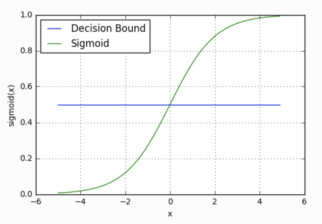
Because the sigmoid function g(z) = 1/(1+e-z), z = WTx+b can perfectly meet the following requirements:
- it assures the output ranges from 0 to 1 (probability).
- the log odds:
is equal to wTx+b (the decision boundary)
The model can be represented as:
- P(Y=1 | x) = g(wTx+b)
- P(Y=0 | x) = 1 - P(Y=1 | x) = 1 - g(wTx+b)
- P(Y=yk | x;w;b) = P(Y=1 | x)yk(1 - P(Y= 1| x))1-yk

Figure 1. Sigmoid Function & Decision Boundary (Image source: ML Cheatsheet)
Parameter Estimation: MLE
Assuming all the training set (N samples) were generated independently, so the likelihood of the parameters can be represented as:
Then, we want to obtain w, b which maximize the log likelihood:
Correspondingly, we try to find w, b to minimize the negative log-likelihood for logistic regression: , which is exactly in the form of cross-entropy error function.
Loss Function & Cost Function
In linear regression, squared error is used to measure the loss between y and for each sample, and sum of squared error to calculate cost function for the whole dataset. While in logistic regression, cross entropy is the substitution.
Loss function:
Cost function:
In the training process, the goal is to minimize the Ein(W), which means to find a spot where ▿Ein(W)=0, when Ein(W) is a continuous convex function. But unlike linear regression, whose ▿Ein(W) is linear, it is hard to calculate ▿Ein(W) for LR directly. So that’s where gradient descent is introduced.
Gradient Descent
To obtain optimal w, b by using gradient descent, we need to iteratively takes steps in the direction of negative of the gradient, update the weights, until certain requirements have been met. (e.g. ||w (k+1)−wk||< ϵ or [J(w(k+1)−J(wk)]< ϵ ). As the conditional likelihood for logistic regression is concave, we can find the global minimum rather than a local minimum.
Repeat:
,
where α is a positive constant learning rate to control the size of each step.
Regularization
Regularization is used for reduce overfitting by adding penalty for large values of w. + λΦ(w)
One way is to add L2 (ridge) norm to the log likelihood:
Φ(w) = (λ would be set as λ/2)
The other is using L1 (lasso) norm:
Φ(w) = |w|
L2-regularized loss function is smooth, meaning the optimum is the stationary point (0-derivative point). L2 can be regarded as weight decay, it won’t make the coefficients become zero. On the contrary, L1 can. Meanwhile, L1 regularization gives you sparse estimates.
Derivative Calculation
Model Interpretation
Before talking about how to interpret LR, let’s take a look at a few terms first.
- Odds v.s. Odds Ratio:
- Odds = probability of event / probablity of non-event. So if odds = 3, then the probability of having that event is twice higher than that event won’t happen.
- Odds ratio = Odds / Odds. Odds explains the risk ratio of having an event vs not, while odds ratio can explain the influence of each single variable on the probability of an event happening or not.
- suppose
- with 1 unit increase in x1, the odds ratio will be
, which is exactly
, meaning with 1 unit change, the odds will multiply by a factor of
.
- suppose
- Logit Function v.s. Sigmoid Function:
- Logit Function is the log of odds. Its output ranges from - \infty to + \infty.
- Sigmoid Function(explained in previous section)

Figure 2. Logit Function (Image source: Wiki)
Experiment: Malicious URL Dection
The dataset contains around 420,000 pieces url records. We want to identify if it’s a bad url.
Table 1
| url | label |
|---|---|
| iamagameaddict.com | bad |
| slightlyoffcenter.net | bad |
So the 1st step is to cut the url into tokens. As the format of a url is kind of fixed: it contains protocol, host name (primary domain) and so on, we can firstly cut the url by ‘.’, ‘/’, and remove some common parts in the url, such as ‘http’, ‘com’, ‘net’. Then, we would use logistic regression to do the prediction.

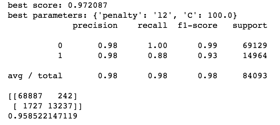
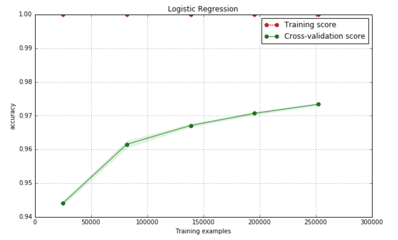
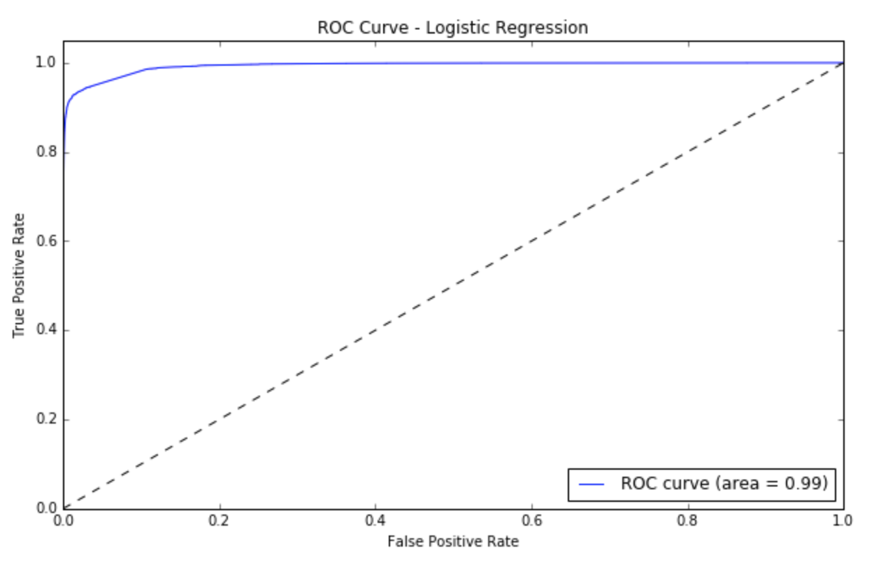
I have used gridsearchCV to find optimal parameters which is l2, with C (equal to 1/λ) set to be 100, then the classificatio accuracy of training set is around 97%, while for the testing set, it can also be up to 95%.


References
[1]. BISHOP, C. M. (2016). PATTERN RECOGNITION AND MACHINE LEARNING. S.l.: SPRINGER-VERLAG NEW YORK.
[2]. Murphy, K. P. (2013). Machine learning: a probabilistic perspective. Cambridge, Mass.: MIT Press.
[3]. http://blog.fukuball.com/lin-xuan-tian-jiao-shou-ji-qi-xue-xi-ji-shi-machine-learning-foundations-di-shi-jiang-xue-xi-bi-ji/
[4]. https://chenrudan.github.io/blog/2016/01/09/logisticregression.html
[5]. http://www.csuldw.com/2016/09/19/2016-09-19-logistic-regression-theory/
[6]. https://hackernoon.com/gradient-descent-aynk-7cbe95a778da


Leave a Comment